
Your monitoring shows CPU hovering at 80%. Prometheus metrics tell you which pods are consuming resources. Your OpenTelemetry pipeline connects traces to logs. Grafana dashboards show the symptoms. But you still can’t answer the most basic question during an incident: which function in your code is actually burning the CPU?
This is the instrumentation tax. You can add more metrics, more logs, more traces. But unless you instrument every function with custom spans (which no one does), you’re still guessing. You grep through code looking for suspects. You deploy experimental fixes and hope CPU drops. You waste hours when the answer should take seconds.
eBPF profiling changes this. It samples stack traces directly from the kernel without touching your application code. No SDK. No recompilation. No deployment changes. You get CPU and memory profiles showing exactly which functions consume resources, across any language, in production, with negligible overhead.
I’m focusing on Parca in this post because continuous profiling is the missing piece in the observability story so far. We covered metrics and traces and security observability. Profiling fills the performance optimization gap.
What eBPF actually solves Link to heading
eBPF lets you run sandboxed programs in the Linux kernel without changing kernel source code or loading modules. For observability, this means you can hook into system calls, network events and CPU scheduling to collect telemetry automatically.
There are three major categories of eBPF observability tools. Cilium and Hubble provide network flow visibility. I covered this in the security observability post when discussing network policy enforcement and detecting lateral movement. Pixie offers automatic distributed tracing by capturing application-level protocols (HTTP, gRPC, DNS) directly from kernel network buffers. You get traces without adding OpenTelemetry SDKs to your code.
But here’s what neither of those do: tell you which functions inside your application are the bottlenecks.
Parca is continuous profiling. It samples stack traces at regular intervals (19 times per second per logical CPU) and aggregates them into flamegraphs. When CPU spikes, you open the flamegraph and see the exact function call hierarchy consuming cycles. Not “this service is slow,” but “json.Marshal in the checkout handler is taking 73% of CPU time because someone passed a 50MB payload.”
Understanding the difference between traces and profiles is important. Traces show request flow across services with timing and context. They’re great for understanding “why is this specific request slow?” Profiles show aggregate behavior over time. They answer “what is my application spending CPU on overall?” You need both. Traces for debugging individual requests. Profiles for optimization and cost reduction.
What eBPF profiling doesn’t give you is business context. It can’t tell you which team owns the hot code path or what the downstream impact is. It won’t correlate profiles with user-facing SLOs. That’s still OpenTelemetry’s job. eBPF collects the low-level truth. OTel normalizes and correlates it with the rest of your observability stack.
This is why I don’t buy the “eBPF replaces instrumentation” narrative. It extends it. You still need explicit instrumentation for ownership metadata, trace correlation and custom business metrics. eBPF gives you the system-level data you can’t easily instrument yourself.
Continuous profiling without the overhead Link to heading
Prometheus scrapes metrics every 15-30 seconds and stores time series. Parca samples stack traces 19 times per second per logical CPU and aggregates them into profiles stored as time series of stack samples. The mental model is similar but the data is different.
When you query Prometheus, you get a number over time. CPU percentage. Request rate. Error count. When you query Parca, you get a flamegraph showing which functions were on the stack during that time window. The width of each box in the flamegraph represents how much CPU time that function consumed relative to everything else.
The sampling overhead is low when properly configured, though actual resource consumption varies significantly based on your workload, number of cores and configuration settings. Compare that to APM agents doing full tracing on every request, which typically add higher overhead depending on the tool and configuration. The reason profiling is cheap is it’s statistical. Missing a few samples doesn’t matter. Over time, patterns emerge even with this sampling approach.
In production, you run Parca as a DaemonSet. Each agent samples its node’s processes using eBPF, then forwards aggregated profiles to a central Parca server. The server stores them and exposes an API for querying. Grafana can display Parca profiles directly, or you use Parca’s own UI.
Integration with OpenTelemetry comes in three flavors. The simplest is running parallel stacks. Parca for profiling, OTel for everything else. You manually cross-reference when debugging. Not ideal but it works.
Better is the Prometheus bridge. Parca can export summary metrics like “top 10 functions by CPU” as Prometheus metrics. Your OpenTelemetry Collector scrapes them alongside everything else. Now your unified metrics backend includes profiling data, even if the flamegraphs still live in Parca’s UI. You can build Grafana dashboards that show CPU metrics from Prometheus next to top functions from Parca, with links to drill into full profiles.
The future path is the OpenTelemetry Profiling SIG. They’re working on standardizing profile data in OTLP, the same protocol that carries metrics, logs and traces today. When that’s ready, Parca and other profilers will export profiles directly to OTel Collectors, and you’ll have true unified pipelines. This started as experimental work in 2024, and while the direction is clear, full production readiness is still evolving.
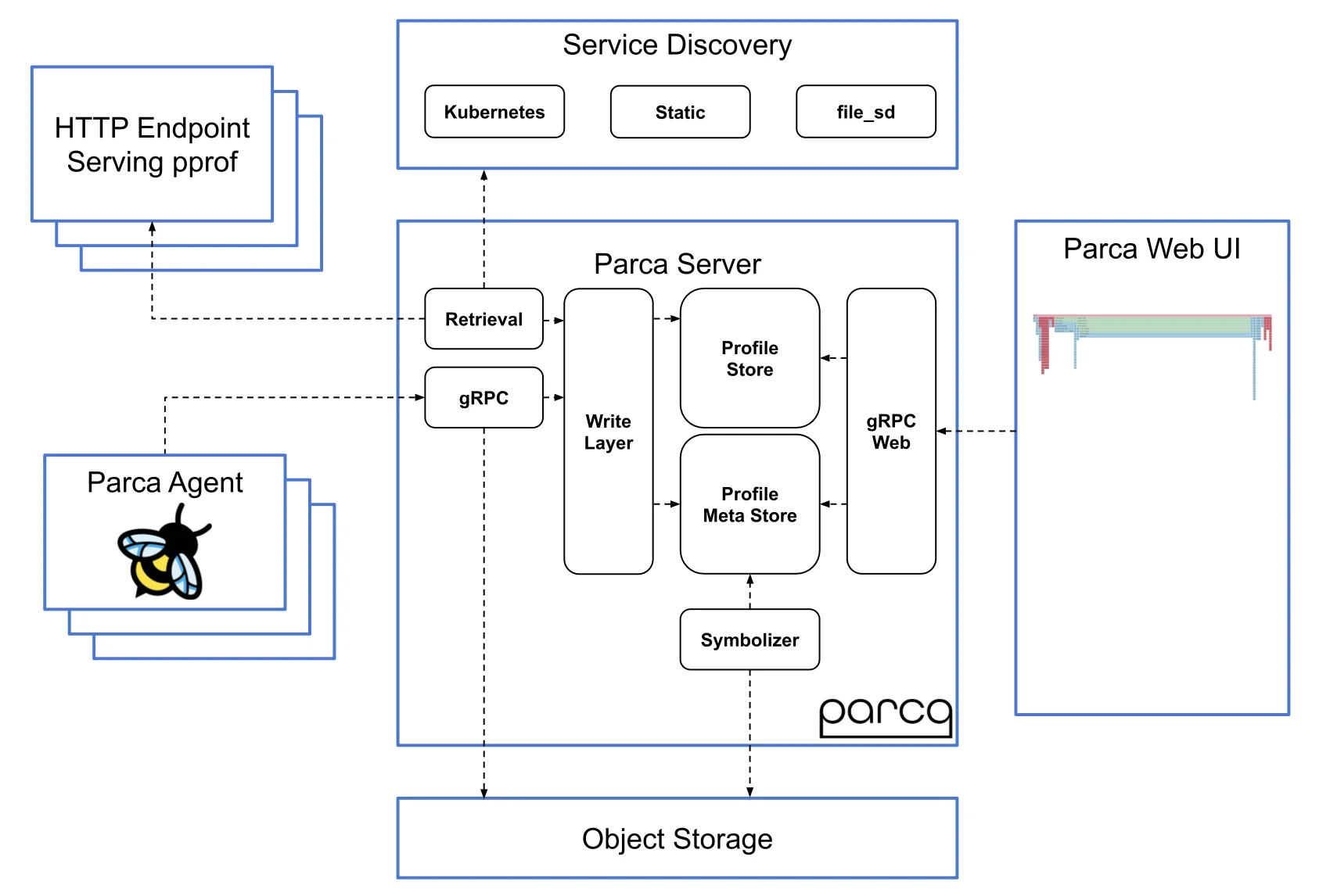 Parca deployment architecture showing DaemonSet agents, central server, and integration options
Should you adopt continuous profiling now Link to heading
Most teams adopt profiling too early. They hear “low overhead visibility” and deploy it cluster-wide before they’ve fixed basic observability gaps. Then they have flamegraphs nobody looks at because alerts still don’t link to runbooks and logs aren’t correlated with traces.
If you haven’t built the foundation from the earlier posts in this series, profiling won’t save you. Fix metrics, logs and trace correlation first. Profiling is an optimization tool, not a debugging tool for mysteries.
That said, some teams need it immediately. If compute costs are a major line item and you’re looking for optimization targets, profiling pays for itself fast. The typical pattern is finding unexpected bottlenecks in libraries you assumed were optimized. JSON serialization, regex matching, logging formatters - these often consume 30-40% of CPU without anyone noticing. Once identified, switching implementations or caching results can cut node counts significantly.
You should adopt profiling if you have recurring performance incidents where the root cause is unclear, especially in polyglot environments where instrumenting every service consistently is hard. eBPF works across languages. A Go service and a Python service produce comparable profiles. You don’t need language-specific APM agents.
Continuous profiling also helps with noisy neighbor problems in multi-tenant clusters. When a pod starts consuming unexpected CPU, profiles show whether it’s legitimate workload growth or runaway code. This is particularly useful for catching infinite loops in production that would take hours to debug with logs alone.
Wait if your team is small and you’re still building observability basics. Profiling adds another system to maintain. The Parca server needs storage. Retention policies need planning. Someone has to own triage workflows when profiles show hotspots. If you don’t have SRE capacity for this, delay.
Skip profiling entirely if you’re running serverless or frontend-heavy workloads where compute cost isn’t significant. Also skip if your organization has strict eBPF policies. Some security teams block eBPF entirely due to the kernel-level access it requires. You’ll need to make the case for CAP_BPF and CAP_PERFMON capabilities before deploying.
Managed Kubernetes makes this easier. Most modern node images support eBPF. EKS, GKE and AKS all work with Parca as long as you’re running recent kernel versions (5.10 or newer recommended, 4.19 minimum). Test in a dev cluster first because older node groups might have restrictions.
The retention question matters for cost planning. Profiling data is smaller than traces but not trivial. A large production cluster generates gigabytes of profile data daily. Most teams keep 30-90 days. Parca supports object storage backends (S3, GCS) so older data can be archived cheaply. Budget accordingly and set lifecycle policies early.
Who owns profiling outcomes? If SREs look at profiles and file tickets for service teams to optimize their code, adoption fails. Service teams need direct access to profiles for their own namespaces. Build dashboards that show “your service’s top CPU functions this week” and make it self-service. Optimization becomes part of the normal development cycle instead of a special SRE project.
What you actually get from profiling Link to heading
Here’s what the process typically looks like. When you first add Parca to a production cluster, profiles show expected patterns. Most CPU goes to business logic, some to JSON parsing, some to database client libraries. Nothing shocking.
The value comes when you filter by the most expensive services measured by node hours per week. Common findings include checkout services burning CPU in logging libraries that pretty-print JSON on every request. Inventory services with caching layers doing more work than just hitting the database. Search services running regex matching in loops that should be precompiled.
Fixing these issues typically yields 20-40% CPU reductions per service. When applied across a cluster, total CPU utilization drops enough to justify downsizing node pools. At scale, even modest optimizations translate to thousands in monthly savings.
The ROI on profiling isn’t always that dramatic but it’s usually positive. Even small optimizations add up when you multiply by request volume. A function that takes 10ms instead of 15ms doesn’t sound impressive until you realize it runs 10 million times a day.
Secondary benefits are harder to quantify but real. HPA oscillation decreases when services have smoother CPU profiles. You get fewer false-positive CPU alerts because you can filter out expected spikes (like scheduled batch jobs). Root cause analysis for performance incidents gets faster when you can jump straight to profiles instead of inferring from metrics.
But here’s where teams screw it up. They deploy Parca, look at flamegraphs during incidents, then do nothing with the information. Profiles become “nice visualizations” that nobody acts on. You need ownership.
I recommend tagging services in Grafana with the team annotation (same one you added to the OpenTelemetry pipeline in the earlier post). Build a weekly report that shows each team’s top CPU-consuming functions. Make it visible. Some organizations add “optimize one hotspot per quarter” to team goals. That’s heavy-handed but it works.
Another mistake is enabling profiling for everything. Start with your most expensive services by compute cost. Profile those for 2-4 weeks. Find and fix the top 3 hotspots. Measure the impact. Then expand to more services. Treat profiling as a targeted optimization tool, not a passive monitoring layer.
Don’t expect profiling to replace distributed tracing. Some teams mistakenly think “we have flamegraphs now, we don’t need traces.” Wrong. Traces show request flow and timing across services. Profiles show where each service spends CPU. A slow request might have a fast profile (it’s waiting on I/O). A fast request might have an expensive profile (it’s CPU-bound but the overall latency is fine). Use both.
If you’re comparing tools, Pyroscope (now part of Grafana after their March 2023 acquisition) is the other major continuous profiler. Parca and Grafana Pyroscope are similar in capability. Parca has stronger eBPF support and remains fully open-source with a cleaner Prometheus integration. Grafana Pyroscope has better multi-tenancy, alerting, and native Grafana Cloud integration. Try both and pick based on your workflow. The profiling concepts are the same.
| Feature | Parca | Grafana Pyroscope |
|---|---|---|
| eBPF Support | Native, first-class | Via agent integration |
| Deployment Model | Self-hosted only | Self-hosted + managed (Grafana Cloud) |
| Prometheus Integration | Native metrics export | Via Grafana integration |
| Alerting | Via external tools | Built-in alerting rules |
| UI/Visualization | Standalone + Grafana | Native Grafana integration |
| Storage Backend | Object storage (S3, GCS) | Object storage + Grafana Cloud |
| Best For | Kubernetes-first, open-source preference | Existing Grafana stack users |
AI tools for performance optimization Link to heading
The intersection of profiling and AI isn’t just about reading flamegraphs. AI coding assistants like GitHub Copilot, Cursor, and Sourcegraph Cody can suggest more efficient implementations when you’re fixing hotspots. Point them at an expensive function from your profile, and they’ll propose alternatives using faster algorithms, better data structures or optimized libraries.
Static analysis tools enhanced with AI can now correlate their findings with runtime profiling data. Tools like Snyk Code and SonarQube are starting to flag performance issues not just based on code patterns but on actual resource consumption in production. When a function appears in profiles as expensive, these tools surface it in code review with severity weighted by real impact.
Cost modeling improves when you combine profiles with infrastructure spending. If a service consumes $800/month in compute and profiling shows 40% of that goes to one function, you know optimizing that function could save $320/month. Multiply across services and you have a prioritized optimization roadmap driven by actual financial impact. Some FinOps platforms are building this correlation automatically.
Automated performance testing tools like k6 and Gatling now integrate with profilers. Run load tests, collect profiles during the test and AI models flag performance regressions by comparing profiles across commits. This catches optimizations that accidentally got rolled back or new code paths that are unexpectedly expensive before they hit production.
For incident response, LLMs help with flamegraph interpretation. Feed a profile into current models like GPT-5, Claude Sonnet and ask “what’s expensive here?” You get a natural language summary pointing to hotspots with context. Faster than training every engineer to read flamegraphs fluently, though you should verify the analysis against the raw data.
ChatGPT Atlas, OpenAI’s new Chromium-based browser with integrated AI, takes this further. When you see an expensive third-party library function in profiles, Atlas can research it in agent mode - pulling documentation, known issues, and optimization guides automatically while you continue analyzing. The browser memory feature learns from your profiling workflows, so it starts recognizing patterns specific to your stack over time. This turns debugging sessions from manual research into assisted investigation.
Adaptive profiling is coming. Instead of sampling all services equally, the profiler learns which services have variable performance and increases sampling there. Services that run stable profiles get sampled less. You get better visibility where it matters while keeping overall overhead low. The eBPF Foundation is driving standardization of these advanced profiling techniques across the ecosystem.
Natural language queries across observability data are improving. “Show me traces and logs related to the high CPU in the payments service” should surface correlated data across metrics, logs, traces and profiles. We’re not quite there yet but the tooling is converging. When this works reliably, debugging shifts from manual correlation to asking questions.
What’s not ready is fully autonomous optimization. AI can suggest fixes based on profile changes, but it can’t understand your business logic or deployment history. It doesn’t know that the hotspot in your service is expected because you just onboarded a major customer. Human judgment still matters. AI proposes, engineers decide.
Guardrails are critical for any AI integration. Redact sensitive symbols or function names before sending profiles to external LLMs. Use self-hosted models or VPC endpoints when possible. Control costs by summarizing first and only sending deltas for analysis. Keep humans in the loop for approval. Log decisions for compliance.
The future vision is eBPF collects unbiased performance data, OpenTelemetry normalizes and correlates it and AI layers on top to spot patterns and point to runbooks. Full production-grade maturity is still 1-2 years out. But the pieces are coming together.
For now, the practical approach is deploying Parca, integrating it with your existing OTel stack via the Prometheus bridge and building workflows where profiles surface during incidents. Start with manual analysis. Add anomaly detection once you understand normal patterns. Experiment with LLM summaries but verify outputs.
Profiling is where your observability stack shifts from reactive (what broke?) to proactive (how do we optimize before it breaks?). Combined with the unified pipeline from the OpenTelemetry post and the security telemetry from the audit logs post, you’re building something close to full visibility.
The next step is turning all this visibility into faster incident resolution. In the next post, I’ll cover SLOs, runbooks and the operational practices that close the loop from signal to action. Because collecting data is the easy part. Using it to ship faster and break less is the hard part.